
Image 1: Hero image
TL;DR: Can a large language model inspect a neural network’s raw, isolated parameters as plain text and reliably determine what the network was trained to do? My tests suggest that while LLMs can perform surprisingly precise calculations at the “edges” of a network (estimating optimizer step counts or finding output correlations), they do not “trace” the computational paths between layers. Instead, they rely heavily on memorized dataset templates (like CIFAR-10) and default framework conventions to fill in the blanks. When these expectations are changed, the models can identify the math but will confidently guess wrong about the semantics—such as recognizing that a satellite feature maps to output 4, but calling it a “frog” because it expects an animal.
I gave a language model the raw weights of a small neural network as plain text, with no tools and no way to run it. The network had been stopped after just three training updates. The model replied that the drift in the weights “matches about 3 Adam steps at a learning rate near 0.001.”
It was right, even though nothing in the prompt mentioned how the network was trained. It got there by noticing batch norm weights sitting between 0.997 and 1.003, and running variances bottoming out just above 0.729—which is 0.9 cubed (0.93).
At first glance, that looks like deep, abstract reasoning in a mathematical space. On closer inspection, however, the model succeeded by leveraging its familiarity with framework defaults—it recognized PyTorch’s default initialization bounds and batch norm’s default momentum of 0.1 and matched the statistics against those known patterns.
Next, I gave it a network trained to 99.57% accuracy on satellite images. The model correctly identified an internal feature that responds to dark green and tied it to output 4. In this dataset, output 4 is “trees,” and the feature really does fire most strongly on trees.
Yet, the model called it “frog.”
This encapsulates the question at the heart of this exploration: Is a language model really tracing weight flows through complex network layers, or is it performing localized calculations at the edges and filling in the gaps with conventions and datasets it already knows? It seems the model can perform real local math at the network’s boundaries (like conv1, batch norm, and fc2), but is relying on memorized priors to make sense of what those numbers mean.
The Claim, and an Inquiry Into Weight Spaces
In November 2026, Rikiya Takehi, Jayden Teoh, Alex Zhang, and Omar Khattab of MIT CSAIL published “Sparks of Weight-Space Programming.” They report that GPT-6 Astra can read and write neural network weights directly, without gradient descent. In one experiment, it named which grid game each of four identically shaped networks was trained on, working from the weights alone.
I wanted to investigate if something less abstract was at play: Is the model actually reasoning through the network’s calculations, or is it matching against datasets, architectures, and templates it already knows? A network with 32×32 inputs and 10 outputs already looks like CIFAR-10 before a single weight is read. If you change what the model expects—such as the label order or the underlying dataset—does the interpretation hold up?
I explored the reading side of this phenomenon using Claude Opus 5.5. Because I did not test GPT-6 Astra, this is an exploration of the underlying mechanism rather than a direct replication of the CSAIL paper.
How I Tested It
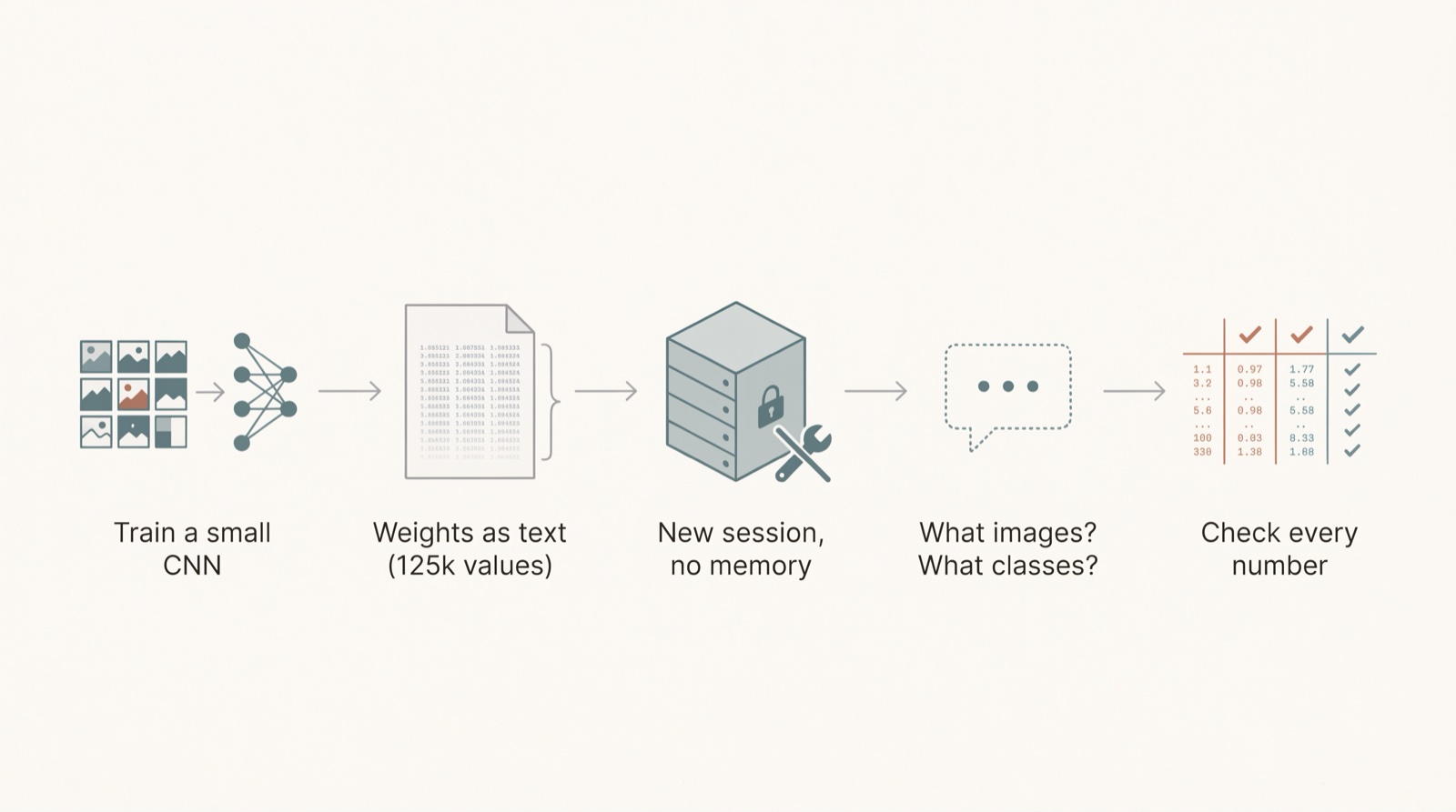
Image 2: Experiment diagram
- Networks: I trained small, unpublished CNNs of about 125,000 weights each, consisting of three blocks of convolution, ReLU, max pooling, and batch norm, followed by two linear layers. Model 1 uses standard filter counts (
16, 32, 64). Model 2 uses unusual filter counts (13, 33, 77). A third Random architecture (62, 68, 25) was chosen by a seeded random draw to match Model 1’s exact parameter count. - Prompt: Each prompt contained the network’s layer formulas followed by every weight as plain text, rounded to 3 decimal places. I omitted the dataset name, class names, normalization constants, and training details.
- Isolation: Every question went to a fresh Opus 5.5 session at extra-high effort, running in a randomly named empty folder with no tools and no memory.
- Verification: I rebuilt each network directly from the prompt text and evaluated it to confirm the model was reading a working classifier. Afterward, verification scripts checked the specific values I could locate in the model’s response against the actual parameters.
- Scoring: All scoring criteria were written down before sending the prompts (excluding the first two trial runs). I ran the pipeline through Claude Code, using subagents for training and Python scripts for verification.
Round 1: A Famous Dataset Looks Like Magic
On CIFAR-10, both sessions named the dataset outright at 90% and 92% confidence, backed by real structural evidence in the weights. In both networks, the dominant sign pattern in the output layer separates outputs {0, 1, 8, 9} from {2, 3, 4, 5, 6, 7}—which corresponds to vehicles versus animals in CIFAR-10’s standard label order.
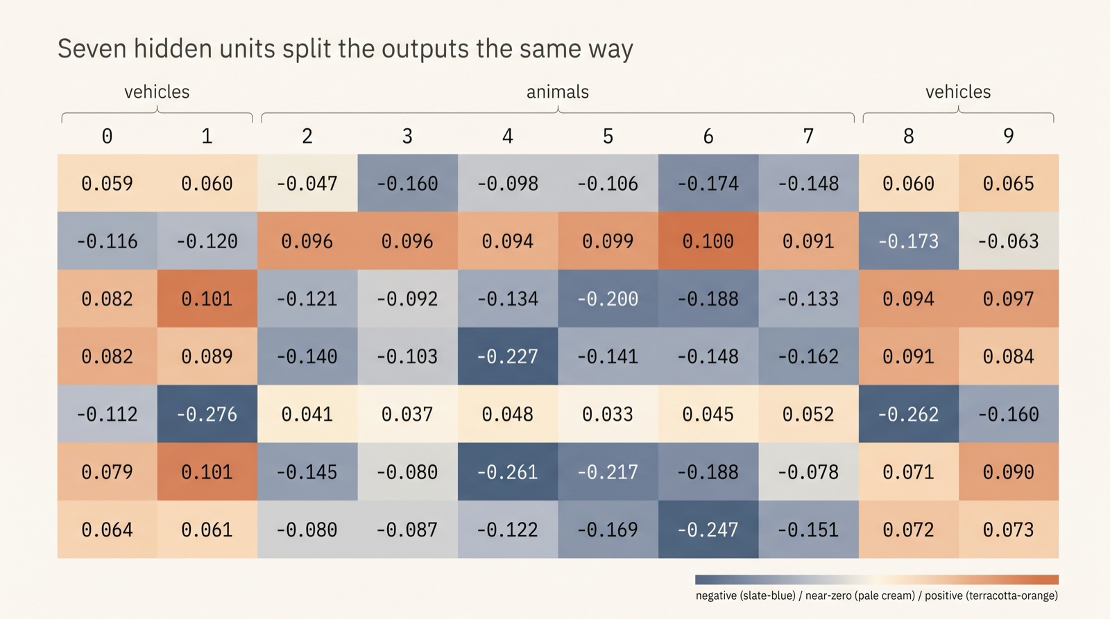
Image 3: The pattern it found
To see whether the model was deriving the classes from the features or leaning on CIFAR-10’s known ordering, I ran two controls on Model 1:
| Control | What I Did | Network Accuracy | Model’s Answer | Confidence |
|---|---|---|---|---|
| None | Original weights | 82.36% | CIFAR-10 | 90% |
| Reordered outputs | Moved vehicles to outputs 2, 4, 5, 7 | 82.37% (renumbered) | CIFAR-10 | 72% |
| Shuffled weights | Scrambled values within each array | 7.78% | CIFAR-10 (best guess) | 45% |
Permuting the output labels broke the model’s class assignments completely. The session still found the mathematical split at its new indices (2, 4, 5, 7), proving it was reading the output layer’s correlation structure. Yet it claimed that “the clusters match the standard label order,” getting every single class pair wrong. It mapped automobile and truck to deer and horse, and described the vehicle cluster as quadrupeds. A reader tracing features through the network to their visual meaning wouldn’t care how the output logits are indexed; a model matching clusters against a memorized CIFAR-10 template does.
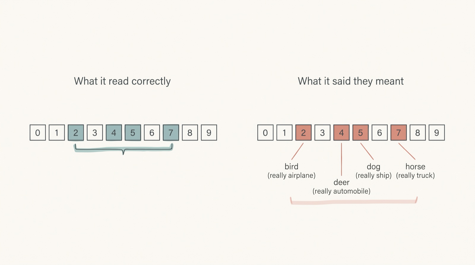
Image 4: Reading against naming
The shuffled control was also telling. Confidence dropped to 45%, and the session rightly noted that the internal structure was gone, adding that its CIFAR-10 guess “relies partly on it being the most common dataset.” However, it never realized the weights had been scrambled, and it still claimed to see evidence of “colour natural images” in pure noise.
Round 2: Less Famous Data
Next, I tested datasets outside the standard CIFAR-10 setup:
| True Dataset | Model 1 Answer | Model 2 Answer |
|---|---|---|
| KMNIST (Japanese characters) | MNIST (80%) | MNIST (85%) |
| Cats vs Dogs | CIFAKE (30%) | Cats vs Dogs (35%) |
| Fast food photos | CIFAR-10 (45%) | CIFAR-10 (50%) |
KMNIST produced the sharpest local deduction. Both sessions ruled out color datasets even though my prompt mistakenly described the input as RGB. They reasoned that when three input channels carry identical grayscale data, they receive identical gradients during training, meaning cross-channel weight differences cannot drift beyond PyTorch’s random-initialization bound of 0.385. Having verified that no channel gap exceeded that threshold, the model inferred a dark background and sparse strokes from the batch norm statistics—and then defaulted to the most famous dataset fitting that profile: MNIST.
On the fast food dataset, neither session mentioned food. The random-architecture network also guessed CIFAR-10 at 60% confidence, with one session noting that its guess “rests on how common it is, not on the weights.”
Round 3: Better Questions, Architecture Controls, and Accuracy
Because a dataset’s name doesn’t test whether the model understands the underlying visual features, I revised the prompt. Instead of asking for a “well-known dataset” name, I asked the sessions to describe what the images show and what each output represents, leaving the dataset name optional.
Does an unusual architecture stop it?
I retrained the random-filter architecture (62, 68, 25) on CIFAR-10 and KMNIST using the revised prompt:
| Dataset | Network Architecture | Network Accuracy | Image Type | Classes in Position | Confidence (Type / Classes) |
|---|---|---|---|---|---|
| CIFAR-10 | Standard (16, 32, 64) | 82.36% | Correct | 10 of 10 | 95% / 90% |
| CIFAR-10 | Random (62, 68, 25) | 83.95% | Correct | 10 of 10 | 92% / 85% |
| KMNIST | Standard (16, 32, 64) | 97.84% | Partial: grayscale strokes, called digits | 0 of 10 | 85% / 65% |
| KMNIST | Random (62, 68, 25) | 97.95% | No answer | No answer | No answer |
The random architecture scored 10 out of 10 on CIFAR-10, though that doesn’t fully exonerate non-standard architectures. While the hidden layer widths were unconventional, the input remained 32×32 and the output remained 10 classes—the exact footprint of CIFAR-10. Those outer dimensions alone heavily anchor the prior: the fast food networks shared the same 32×32×3-to-10 shape and were consistently labeled CIFAR-10, and even a 6-class SAT-6 network at 32×32 was interpreted as the six animal classes of CIFAR-10. (The KMNIST random session produced no answer after exhausting its full output token budget on internal reasoning, and a follow-up continuation hit an unspecified safety stop.)
Notably, the standard CIFAR-10 session explicitly drew the line between what it could calculate and what it was recalling from memory:
“The weights show which outputs pair up, but not which member is which. Telling cat from dog, deer from horse, airplane from ship, or automobile from truck relies on the standard CIFAR-10 order.”
Does network accuracy matter?
Because the fast food classifier was both an obscure dataset and weakly trained (~55% accuracy), it couldn’t separate dataset familiarity from model quality. SAT-6 can. It is a less-known dataset of 28×28 satellite image patches, resized to 32×32 across six classes: barren land, building, grassland, road, trees, and water. It is also easy to learn, reaching roughly 90% accuracy from just 24 training images. To create a low-accuracy counterpart with the exact same data, architecture (Model 2), and prompt, I stopped training after three updates:
| SAT-6 (Model 2) | Test Accuracy | Macro F1 | Image Type | Classes in Any Position | Name Given | Confidence (Type / Classes) |
|---|---|---|---|---|---|---|
| High accuracy | 99.57% | 99.51% | Wrong: animal photos | 0 of 6 | CIFAR-10, animal classes | 70% / 45% |
| Low accuracy | 36.01% | 22.91% | Partial: scenes (“only a guess”) | 4 of 6 | Unknown | 30% / 3% |
Having a near-perfect 99.57% network did not help the model recognize satellite imagery; it only made the session more confident in a fabricated story about animal photos. While the low-accuracy network technically scored 4 out of 6 classes in any position, that came from a generic list of outdoor scene categories that the model itself caveated as a “guess from priors” at 3% confidence.
Comparing what the high-accuracy session extracted from the weights against ground truth shows exactly where the reasoning goes off the rails:
| What the Session Read | What Is True in the Network | What the Session Concluded |
|---|---|---|
| A “dark green” feature favors output 4 | Fires most on trees; output 4 is trees | Output 4 is frog |
| Outputs 1 and 3 form a strong pair (+0.54) | Outputs 1 and 3 are building and road | Cat and dog |
| A “blue” feature favors output 0 | Fires most on grassland and road (below average on water) | Output 0 is bird |
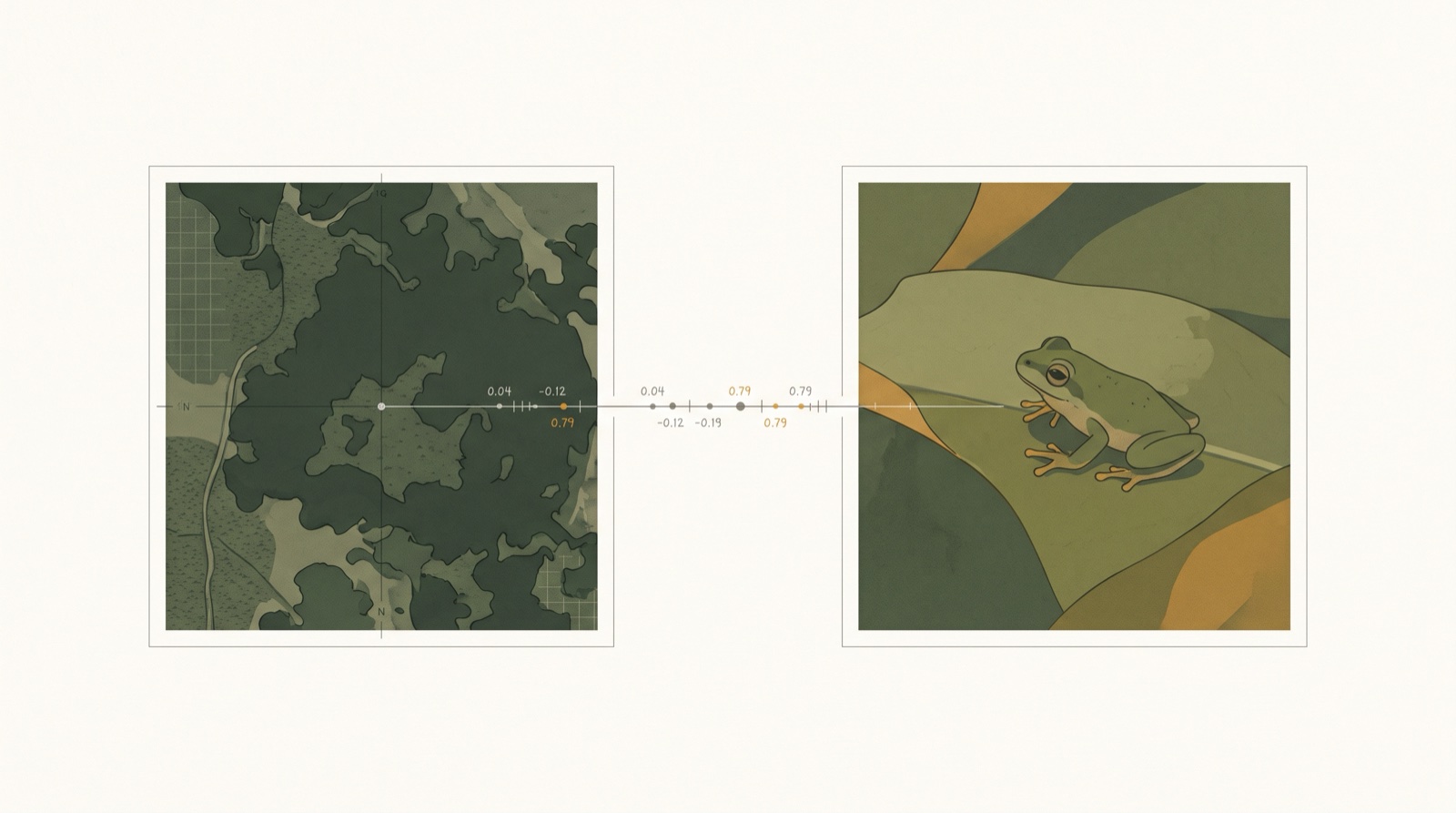
Image 5: Same reading, wrong meaning
The model found genuine low-level and output-level correlations, but without a memorized template for SAT-6, it forced those features into the nearest familiar category: CIFAR-10 animals.
It Isn’t Following the Weights
Tracing a weight flow means following how signals propagate from the input pixels through every intermediate layer to the output logits. In their own words, the sessions never did that:
- “I found nothing here that identifies the dataset, and I did not trace these features through to the outputs.” (CIFAR-10, standard)
- “I read conv2 only for kernel shape, did not trace conv3 or fc1 in detail.” (CIFAR-10, random)
- “I worked by hand and did not trace most of conv2 and conv3.” (KMNIST)
- “I traced class evidence for only 7 of the 77 a3 channels.” (Cats vs Dogs)
- Calculated rough channel-to-output effects “using only 10 to 18 of the 78 hidden units.” (SAT-6)
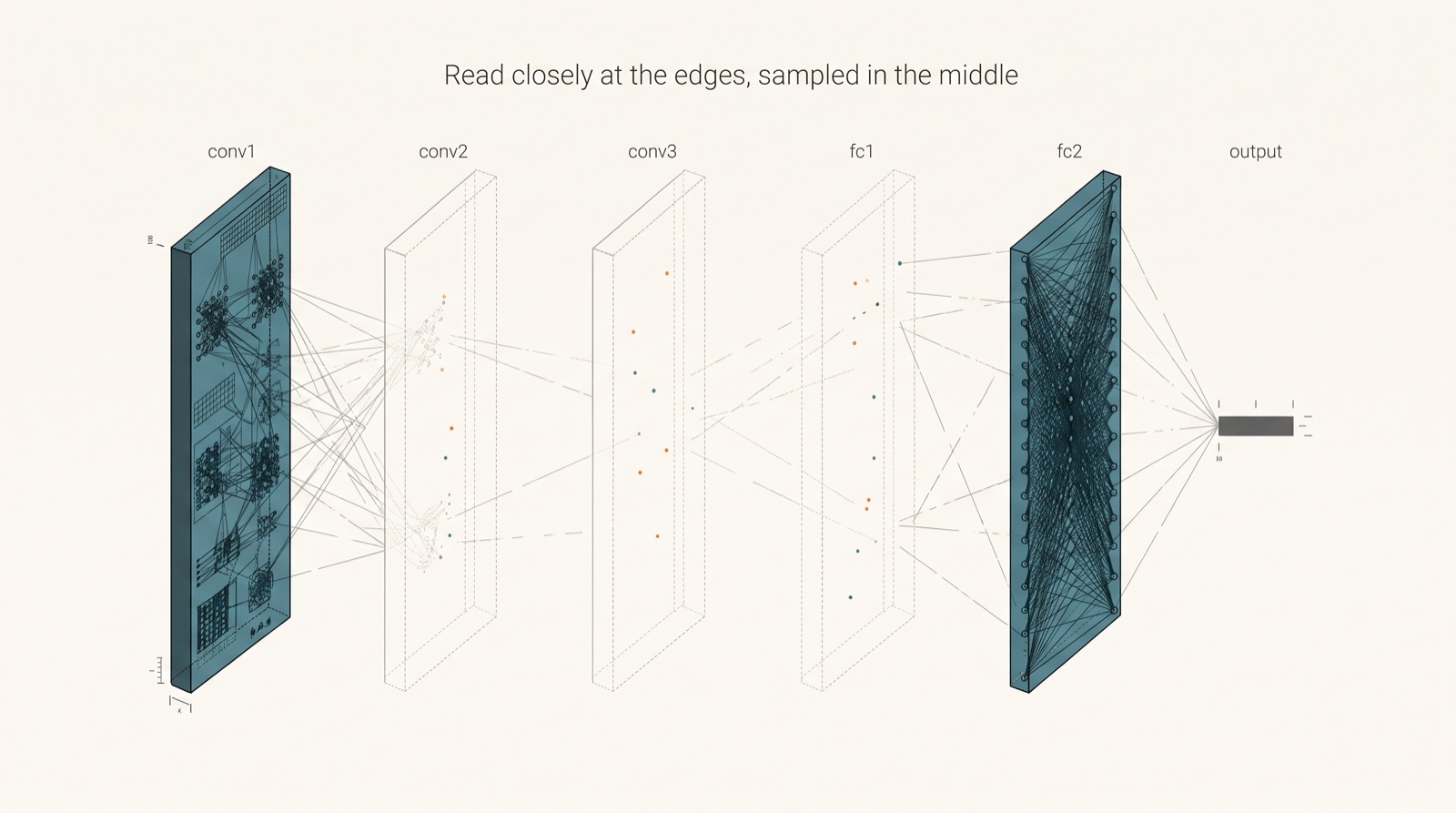
Image 7: Where the sessions actually looked
Whenever a session did attempt to make claims based on multi-layer tracing, those claims failed verification against the actual weights:
- “Top-heavy” spatial evidence: One session sampled 10 of the 78 hidden units, claimed class evidence was concentrated at the top of the image, and used that to argue for “heads and ears.” Across all 78 hidden units, however, spatial importance actually peaks in the second row (
0.109, 0.144, 0.107, 0.092). - Misread deep features: The SAT-6 session labeled a deep feature “blue” and used it to argue that output 0 was bird(which is interesting that it thinks blue is related to bird). When run on the dataset, that feature fires primarily on grassland and road, and activates below average on water.
- Indexing errors: Another session quoted real weight values from the prompt, but off-by-two indexing assigned them to the wrong input channels, invalidating the deduction built on top of them.
Where the Evidence Lands
| Hypothesis Component | Verdict | Deciding Evidence |
|---|---|---|
| Label order breaks it | Supported | Renumbered outputs kept their memorized CIFAR-10 meanings; all 9 named class pairs were wrong. |
| Input and output shape bias the guess | Supported (indirectly) | Same-shape fast food became CIFAR-10. Every network used 32×32 inputs, so input dimensions weren’t varied. |
| It isn’t following weight flows | Supported | Sessions explicitly admitted skipping middle layers, and claims based on partial tracing failed script checks. |
| It leans on famous datasets | Supported | KMNIST became MNIST, and 99.57%-accurate SAT-6 became CIFAR-10 animal photos. |
| Non-standard architectures break it | Unresolved | Unusual hidden layer widths didn’t break CIFAR-10 recognition, but input/output dimensions stayed standard. |
| Higher accuracy helps recognition | No evidence (on one pair) | On SAT-6, 99.57% accuracy increased confidence in the wrong answer rather than improving correctness. |
| Weight editing works the same way | Not tested | Editing runs were stopped before completion. |
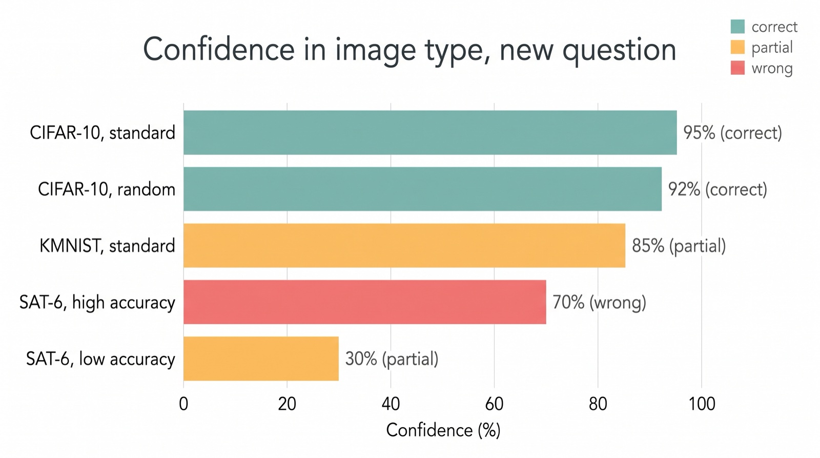
Image 6: Confidence in image type
The evidence points to a consistent conclusion: language models can spot real statistical patterns in raw parameters, but they interpret those patterns by matching them against familiar models, datasets, and framework defaults.
It seems the model can calculate the parameters’ specific local properties—determining initialization scales, estimating optimizer step counts, and discovering output correlation patterns—but when asked to synthesize those patterns into semantics, it reaches back to the templates it knows. It performs impressive local math at the network’s boundaries, but depends on its internal training prior to guess what the math is trying to accomplish.
What this doesn’t show
It doesn’t refute the MIT CSAIL paper. I tested a different model (Claude Opus 5.5 vs. GPT-6 Astra) on a single task. Their claims about initializing networks from scratch and surgically editing language models are untouched by these results.
The experimental setups differ in a crucial way. In Experiment 1 of the MIT paper, the prompt explicitly labeled what each input channel represented (e.g., “agent” and “reward targets”), and the first-layer weights mapped directly onto those labeled grid coordinates. My prompts gave no semantic labels for the outputs, and raw RGB pixels don’t carry symbolic channel labels.
Sample sizes are tiny. Most configurations were run once, on a single random seed, with a single model.
Weight editing remains untested.
Some things to note:
- Three sessions hit the output ceiling. The shuffled CIFAR-10 run, the KMNIST random-architecture run, and the high-accuracy SAT-6 run all exhausted their 128,000-token limit and received an automated “resume” prompt, making those transcripts slightly different from the single-turn sessions.
Ideas for Further Testing
If you wanted to continue testing the bounds of what LLMs can read in weight-space, here are several angles that could further clarify their actual tracing capabilities vs. their pattern priors:
- A forward-pass flow test: Give the model a network and a single concrete input tensor, and ask for the exact output logits. A model that can genuinely trace weight flows should get close; a local pattern-matcher won’t.
- A shape and order test: Train a random architecture on CIFAR-10 resized to a non-standard input resolution with permuted class labels. If it still identifies vehicles and animals and assigns the right class names, it isn’t relying on shape or label order.
- Non-default training hyperparameters: Initialize weights with a non-standard distribution and change the batch norm momentum. If the model still reconstructs the training dynamics, it isn’t just leaning on PyTorch defaults.
- Tool use: Give the model Python in the same isolated setup. If it writes code to trace intermediate feature maps and correctly identifies obscure datasets like SAT-6, the bottleneck was mental arithmetic rather than weight-space comprehension.
- Blind weight editing: Test whether the model can improve accuracy on an unseen network without gradient descent or training data.
- Multi-seed repeats across frontier models: Run multiple seeds per condition across both GPT-6 Astra and Claude Fable.
Appendix: Full Results and Prompt
Original Question (Naming the Dataset)
| True Dataset | Network | Test Accuracy | Model Answer | Confidence | Score |
|---|---|---|---|---|---|
| CIFAR-10 | Model 1 | 82.36% | CIFAR-10 | 90% | Correct (no preset rule) |
| CIFAR-10 | Model 2 | 82.28% | CIFAR-10 | 92% | Correct (no preset rule) |
| CIFAR-10 (reordered) | Model 1 | 82.37% | CIFAR-10 | 72% | Fail |
| CIFAR-10 (shuffled) | Model 1 | 7.78% | CIFAR-10 (best guess) | 45% | Pass |
| KMNIST | Model 1 | 97.84% | MNIST | 80% | Partial |
| KMNIST | Model 2 | 97.58% | MNIST | 85% | Partial |
| Cats vs Dogs | Model 1 | 87.70% | CIFAKE | 30% | Neutral |
| Cats vs Dogs | Model 2 | 87.95% | Cats vs Dogs | 35% | Neutral |
| Fast food | Model 1 | 54.67% | CIFAR-10 | 45% | Neutral |
| Fast food | Model 2 | 52.67% | CIFAR-10 | 50% | Fail |
| Fast food | Random | 58.00% | CIFAR-10 | 60% | Fail |
Revised Question (Describing the Dataset)
| True Dataset | Network | Test Accuracy | Image Type | Classes in Position | Classes in Any Position | Name Given |
|---|---|---|---|---|---|---|
| CIFAR-10 | Standard | 82.36% | Correct | 10 of 10 | 10 of 10 | CIFAR-10 |
| CIFAR-10 | Random | 83.95% | Correct | 10 of 10 | 10 of 10 | CIFAR-10 |
| KMNIST | Standard | 97.84% | Partial | 0 of 10 | 0 of 10 | MNIST |
| KMNIST | Random | 97.95% | No answer | No answer | No answer | No answer |
| SAT-6 | Model 2 (high acc.) | 99.57% | Wrong | 0 of 6 | 0 of 6 | CIFAR-10, animals |
| SAT-6 | Model 2 (low acc.) | 36.01% | Partial | 0 of 6 | 4 of 6 | Unknown |
(Note: I also ran SAT-6 Model 1 at low accuracy [63.36%]. It declined to guess, listing every class as unknown at 1% confidence while correctly inferring ~3 Adam steps. Because its high-accuracy counterpart was stopped before completion, Model 1 was omitted from the SAT-6 comparison table.)
- Training protocol: Adam (
lr = 1e-3), batch size 128, learning rate halved on plateau, early stopping with patience 10, up to 100 epochs, seed 0. Images were resized to 32×32, except KMNIST, which was padded from 28×28 to 32×32 and replicated across three channels. - Datasets tested: CIFAR-10, KMNIST, Cats vs Dogs, Fast Food Classification, and SAT-6.
The Prompt (Revised Version, SAT-6 Model 2)
Other networks differed only in channel counts and output dimensions. The original Round 1–2 question ended by asking: “Which dataset was it trained on?” and “If it resembles a well-known dataset, give that dataset’s name.”
THE INPUT
The network sees a 32 x 32 RGB image. Rows are numbered 0 (top) to 31 (bottom) and columns 0 (left) to 31 (right). Input channel 0 is red, channel 1 is green and channel 2 is blue. Before entering the network, each channel was standardized by subtracting a fixed mean and dividing by a fixed standard deviation. Those constants are not given here.

THE OUTPUTS
The network outputs 6 numbers (logits), one per class. The class probabilities are the softmax of these logits. What each output stands for is not given.

THE NETWORK
A convolutional image classifier. Every convolution has a 3 x 3 kernel, stride 1 and padding 1. Every max pool has a 2 x 2 window and stride 2.
  a1 = bn1(maxpool(relu(conv1(x))))          conv1: 3 to 13 channels, a1 is 13 x 16 x 16
  a2 = bn2(maxpool(relu(conv2(a1))))         conv2: 13 to 33 channels, a2 is 33 x 8 x 8
  a3 = bn3(maxpool(relu(conv3(a2))))         conv3: 33 to 77 channels, a3 is 77 x 4 x 4
  f = flatten(a3)                            1,232 numbers
  h = relu(f @ fc1.weight + fc1.bias)        fc1.weight: 1,232 x 78, fc1.bias: 78
  logits = h @ fc2.weight + fc2.bias         fc2.weight: 78 x 6, fc2.bias: 6
A convolution's weight has the shape (filter, input channel, kernel row, kernel column).
Batch norm is applied per channel, using fixed statistics: bn(a) = (a - running_mean) / sqrt(running_var + 0.00001) * weight + bias.
Flattening follows f[i], where i = channel * 16 + row * 4 + column.
During training only, dropout with p = 0.3 was applied to h.
The network has 124,098 trained parameters and 246 batch norm running statistics. It was trained with supervised learning to classify images from one image dataset into 6 classes.

QUESTION. The weights below belong to one image classifier that was trained with supervised learning on one image dataset. Work from the weights to describe that dataset: what kind of images it contains and what its 6 classes are. A dataset name is optional. If the weights do not support an answer, say so and give a low confidence. You have no tools: no code execution, no calculator, nothing to run. This is a single response.

Answer in this order:
Observations: <what you see in the weights, layer by layer; quote the weights you rely on>
Reasoning: <which kinds of images and classes fit these observations, which are ruled out, and why>
Image type: <what the images show, in one or two sentences>
Classes: <one line per output, from output 0 to output 5, giving what you think it stands for>
Dataset name: <a name if you have one, otherwise unknown>
Confidence in image type: <0-100>%
Confidence in classes: <0-100>%

THE NETWORK'S WEIGHTS
Values rounded to 3 decimals.

conv1.weight, shape 13 x 3 x 3 x 3: one line per (filter, input channel), 9 values per line, in kernel row order
{{conv1.weight}}

conv1.bias, shape 13:
{{conv1.bias}}

(The same format continues for bn1, conv2, bn2, conv3, bn3, fc1 and fc2.)
References
Rikiya Takehi, Jayden Teoh, Alex Zhang, and Omar Khattab. Sparks of Weight-Space Programming: LLMs can natively read & write neural network weights. November 2026.
Cite this Article
@misc{ahmed2026llmweights,
  title        = {{Can an {LLM} Actually Reason and Program about Neural Network's Weights or is it just memorization on steroids? {Exploring} 'Weight-Space Programming'}},
  author       = {Ahmed, Nazmus Sakib},
  year         = {2026},
  month        = nov,
  howpublished = {\url{https://sakibbai.com/posts/2026-11-05-llm-weight-space-programming/}},
  note         = {Blog post, Latent Space}
}